Heart Disease UCI

This database contains 76 attributes, but all published experiments refer to using a subset of 14 of them. In particular, the Cleveland database is the only one that has been used by ML researchers to this date. The goal of this project is to find trends in heart data to predict certain cardiovascular events or find any clear indications of heart health

# General packages
import pandas as pd
import numpy as np
import matplotlib.pyplot as plt
import seaborn as sns

#Modelling 
import statsmodels.formula.api as smf

# Loading data 
df = pd.read_csv("C:/Users/Stevie/Data_Analysis/Regressions/heart.csv")

# age in year
# sex (1 = male; 0 = female)
# chest pain type
# trestbps : resting blood pressure (in mm Hg on admission to the hospital)
# chol: serum cholestoral in mg/dl
# fbs (fasting blood sugar > 120 mg/dl) (1 = true; 0 = false)
# restecg resting electrocardiographic results
# thalach : maximum heart rate achieved
# exercise induced angina (1 = yes; 0 = no)
# ST depression induced by exercise relative to rest

Plots

import warnings
warnings.filterwarnings('ignore')

f = plt.figure(figsize=(14,6))

ax = f.add_subplot(121)
sns.distplot(df['thalach'],bins=40)
plt.title('Distribution of maximum heart rate')
plt.xlabel('Heart Rate')


ax = f.add_subplot(122)
sns.distplot(np.log10(df['thalach']),bins=40,color="r")
plt.title('Distribution of $log$(maximum heart rate)')
plt.xlabel('Heart Rate')

f2 = plt.figure(figsize=(14,6))

df['Gender'] = df['sex']
df.loc[df.Gender==0,'Gender'] = "Female"
df.loc[df.Gender==1,'Gender'] = 'Male'

df['Angina'] = df['exang']
df.loc[df.exang==0,'Angina'] = "Yes"
df.loc[df.exang==1,'Angina'] = 'No'

df['t'] = df['target']
df.loc[df.target==0,'t'] = "No_Heart_Disease"
df.loc[df.target==1,'t'] = 'Have_Heart_Disease'

ax = f2.add_subplot(121)
sns.violinplot(x='Gender',y='chol',data=df,ax=ax)
plt.title('Violin Plot: \n cholestoral level for both Male/Female')

ax = f2.add_subplot(122)
sns.violinplot(x='Angina',y='chol',data=df,ax=ax)
plt.title('Violin Plot: \n cholestoral level for both Male/Female')

plt.figure(figsize=(14,6))
sns.boxplot(x='restecg',y='chol',hue='Gender',data=df)
plt.legend(fontsize=11)
plt.xlabel('Resting electrocardiographic results (values 0,1,2)')
plt.ylabel('Cholestoral level')
plt.title("Boxplot: \n Resting electrocardiographic results and cholestoral levle for Male and Female ")

del df['Gender']
del df['Angina']

d = df[['Gender','cp','chol','t']]
d2 = d.melt(id_vars=['Gender','cp','t'])
d2 = d2.groupby(['Gender','cp','t'])[['value']].count()
d2 = d2.pivot_table(
            index=['Gender','t'],
            columns='cp',
            values='value',
)

d2.plot(kind='barh',stacked=True,figsize=(14,6),title="Different types of chest pain per patient/gender ",color=['#1A374D','#406882','#6998AB','#B1D0E0'])
plt.xlabel('Number of People')
plt.legend(['Type 0','Type 1','Type 2','Type 3'])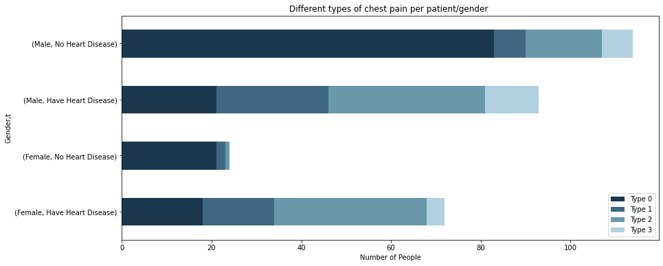

plt.figure(figsize=(14,6))
plt.hist((df[df['target']==0].age,df[df['target']==1].age),color=['#1A374D','#406882'])
plt.legend(['No Heart Disease','Have Heart Disease'],fontsize=12)
plt.xlabel("Age")
plt.ylabel('Number of people')
plt.title("Histogram: \n Age distribution of different type of patients (with and without heart disease)")

plt.figure(figsize=(14,8))sns.heatmap(df.corr(),annot=True)
plt.title('Correlation Heatmap')

Looking at the correlation plot, it seems like chest pain and maximum heart rate has a great impact on wheather a patient has heart disease

Modelling

# Processing categorical columns and creating dummies
n = ['t','cp']
df_encode = pd.get_dummies(df,
                           prefix= 'd',
                           prefix_sep='_',
                           columns= n,
                           drop_first=True, #remove if you want 0 to be a true value
                           dtype='int8')

mod3 = smf.ols(formula='target~age+sex+d_1+d_2+d_3+exang',data=df_encode)
res3 = mod3.fit()
print(res3.summary())

Analysis

All p values are below 0.05, which indicates that all of my variables are significant. If we assume age is continous, it means that a patient being older by 1 year will decrease the log odds of a person having heart disease. This is agaisnt my hypothesis that an older person is more likely to have heart problems.

As for other variables, a patient having type 0 chest pain is more likely (log odds) to have heart problems. The log odds for all other chest pain type are more or less the same (0.36-0.37).

Also, if a patient is experiencing an agina, they are more likely to be a patient with heart disease.

R_sqaured indicates that my model explains 40% variation of the dependent variable. Thus, I suspect that a better model could be used.

Homoskedasticity

test = sms.het_breuschpagan(res3.resid, res3.model.exog)
lzip(names, test)

# p - value < 0.05
[('Lagrange multiplier statistic', 16.622046172773267),
 ('p-value', 0.010777402900715863),
 ('f-value', 2.863422039177654),
 ('f p-value', 0.009997680063051234)]

Normality

sns.distplot(res3.resid)

Additional Plots

import statsmodels.api as sm
fig = plt.figure(figsize=(14, 10))
sm.graphics.plot_ccpr_grid(res3,fig=fig)
fig.tight_layout(pad=2.0)